
I bought a second hand M-DAC a while ago to have a well-known commercial reference in terms of measurements and sound. After teardown it is time for measurements. The first part focused on the base performance and this second part dives into the digital filters and their impact on measurements.
In the first part all base performance measurements were carried out using ‘Optimal Spectrum’ filter but here we will have a look at the differences between the seven filters M-DAC offers. This post focuses on measurements and technical aspects of the filters, not their sonic characteristics which are always subjective.
Digital filtering
Basic understanding of filters and especially digital filtering is required to understand how they change signal. Concepts like oversampling, Nyquist frequency, aliasing/folding, and image frequencies are important here. I have touched the topic a bit in another post in the past where I compared slow and sharp rolloff filters of PCM1794A DAC chip. One brief explanation of oversampling interpolating DACs by Analog can be found here.
Filters change signal and the changes can be illustrated in time or frequency domain. Time and frequency domain representations are two sides of the same thing, and optimising one deteriorates the other. Some M-DAC filter names refer to these directly, such as ‘Optimal Transient’ and ‘Optimal Spectrum’. The former optimises the time domain (transient response), while the latter optimises the frequency domain (frequency spectrum). In a way these can be considered as the two extremes and the rest of the filters are somewhere in between – although as usually, it is not quite as simple.
Digital filters in M-DAC
It is common for better DACs to have more than one filter option but seven is an ample number of options. Here are the names of the filters and what the user manual tells about them:
‘Optimal Transient’, ‘Optimal Transient XD’, and ‘Optimal Transient DD’
“Optimal Transient filters exhibit no ringing – the transient nature of the music is preserved. Although exhibiting poorer performance in technical measurements, sound from this type of filter has a purity and ‘naturalness’ that more than compensates for the lack of technical specifications. There are three Optimal Transient Filters. They exhibit identical frequency and time domain response but the internal structure of the filters varies, resulting in small but perceptibly different sonic nuances.”
‘Sharp Rolloff’
“Typifies industrial standard characteristics (-6 dB at ½ Fs with significant time-domain ringing) and is included here for comparison purposes.”
‘Slow Rolloff’
“Starts rolling off at a lower frequency than the Sharp Rolloff filter but has a gentle rate of attenuation and significantly less time-domain ringing”.
‘Minimum Phase’
“Has a gentle attenuation slope similar to the Slow Rolloff option, however it exhibits no pre-ringing in the time domain. It can be likened to an analogue filter applied in the digital domain.”
‘Optimal Spectrum’
“A digital filter which implements sampling theory and is designed for near perfect technical response in the frequency domain. This filter also has time-domain pre-ringing which can lead to listener fatigue”
Comments on these filters
Just based on the descriptions it is already clear why ‘Optimal Spectrum’ was used for performance measurements. It simply gives the best technical results, as stated. Otherwise, it seems that optimised time-domain has been the goal here; optimising transient response is seen as more natural. Some consider ringing in digital filter response unwanted and unnatural. This is true especially for pre-ringing; after all, it means pre-response to something that has not been happened yet. We will see these later in the measurements.
Measurements
I took the M-DAC to my work where I have access to Audio Precision analysers. The measurements of this part have been carried out with APx585. I created a measurement sequence containing loads of single-point measurements and sweeps. This sequence was then repeated with different filter settings to gather the data.
Coaxial input, 48 kHz sample rate, and balanced output was used for all measurements and M-DAC set in DAC-mode (as opposed to preamplifier mode) with full 0 dB gain.
Specifications and measurement results using ‘Optimal Spectrum’ filter were shown in part 1 and that gives the baseline performance for the device. These results are shown here again as a reference point.
Common notes on all filters
In terms of crosstalk, noise level, gain, and therefore SNR and dynamic range, there are no differences between the filters.
Measurement results
There are loads of data which has been organised by parameters. If you want to skip some graphs and see the real differences between filters, browse to FFTs and scope plots for frequency and time domain differences.
Optimal Transient filters have been grouped as one to save some space as some results are fairly identical across these.
THD+N vs amplitude
One would think that distortion and noise are determined by the DAC IC output stage and M-DAC output stage. However, there are differences between filters, and oddly between left and right channels. Whether this is typical or only something on this unit, I cannot say. I guess potentially higher frequency components could excite some form of distortion that create differences between filters but you would imagine this to happen on both channels.
Optimal Spectrum filter
Slight variation between channels.
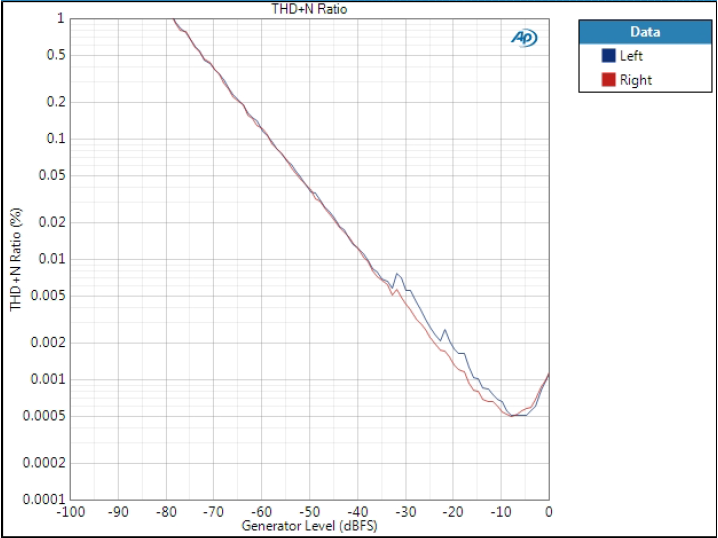
Optimal Spectrum, THD+N ratio
THD+N level is shown only for this one filter as it is basically the same as THD+N ratio except that it shows noise level; however, noise is equal to all filters.
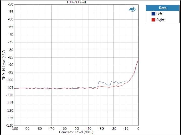
Optimal Spectrum, THD+N level
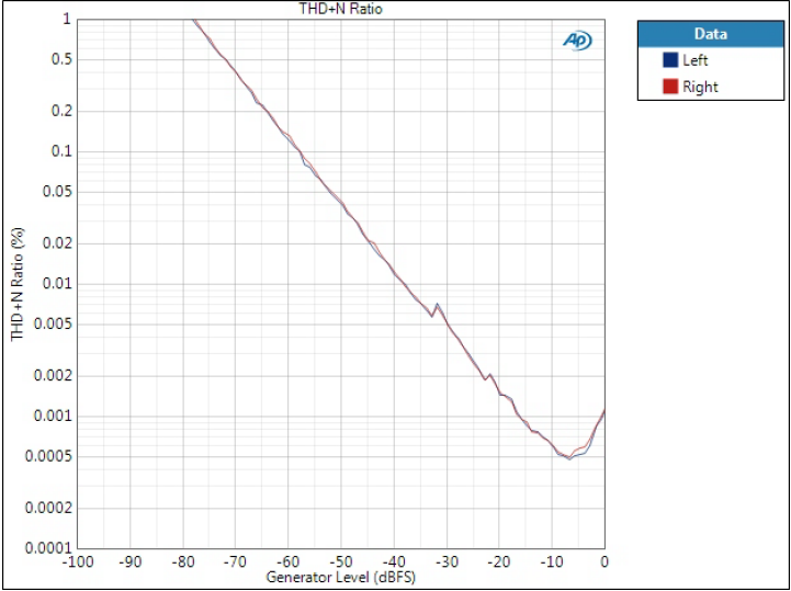
Optimal Transient filters
Here we see clear differences between left and right channels. However, here the right channel is weaker, while in Optimal Spectrum filter left channel had some variation. Anyway, I would not worry about these. Interesting though.
Interesting also that Optimal Transient DD differs from the two – and we will see similar pattern in FFTs.
Optimal Transient, THD+N ratio
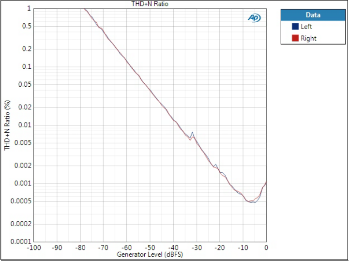
Optimal Transient DD, THD+N ratio
Optimal Transient XD, THD+N ratio
Minimum Phase filter
Minimum Phase, THD+N ratio
Sharp rolloff filter
Sharp Rolloff, THD+N ratio
Slow rolloff filter

Slow Rolloff, THD+N ratio
Frequency response
The effects of the filter can be seen at the end of the audio band as some filters start rolling off earlier than others.
Optimal Spectrum filter
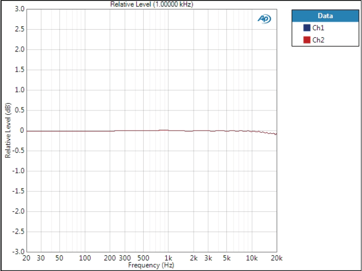
Optimal Spectrum, frequency response
Optimal Transient filters
All three filters have identical frequency response which differs significantly from Optimal Spectrum. These filters have very slow rolloff and it starts early.
Optimal Transient filters, frequency response
Minimum Phase filter
Almost like Optimal Spectrum but we can see sharp cutoff just before 20 kHz.
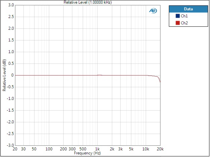
Minimum Phase, frequency response
Sharp rolloff filter
Sharp Rolloff, frequency response
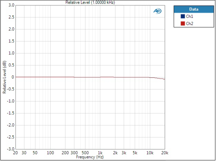
Slow rolloff filter
This also starts rolling off well before 20 kHz.

Slow Rolloff, frequency response
Delay
Delay itself does not matter but it tells something about the length of the filter.
All these are 48 kHz sample rate, and filter length is proportional to the sample length.
- Optimal Spectrum: 1042 μs
- Optimal Transient: 1042 μs
- Optimal Transient DD: 1063 μs
- Optimal Transient XD: 354 μs
- Minimum Phase: 375 μs
- Sharp rolloff: 1042 μs
- Slow rolloff: 438 μs
FFT spectrum, 1 kHz
This is where things get interesting.
This is a 1 kHz tone at -20 dBFS level so there should not be much distortion from the output stage but more revealing the filter characteristics.
The bandwidth of this measurement is 96 kHz and as sample rate is 48 kHz, we should look at two different things. First, what is in the audio band until 20 kHz. This is what is typically measured and for filters made measurements in mind this should be all clean with only the 1 kHz tone.
The second thing is to watch the folding (or image) products. This is an oversampling DAC (as almost all of them) so the fundamental sample rate is a lot higher than 48 kHz, hence we can use digital filtering (which this whole post is about) above 48/2 kHz – and that is why it is used in the first place. When signal is 1 kHz and sample rate 48 kHz, these tones are present at 47 kHz, 49 kHz, and 95 kHz in the shown bandwidth of 96 kHz. Filter characteristics then define how high these tones are and what else happens around them.
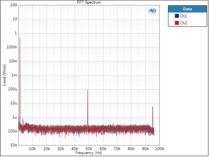
Optimal Spectrum filter
This is what this type of filter is made for. FFT still easily reveals the folded tones but attenuation is around 100 dB.
Unfortunately I forgot to change the scale from Vrms to dBV here.

Optimal Spectrum, 1 kHz FFT
Optimal Transient filters
And this is where we see the biggest contrast in comparison to the previous graph.
Let’s first look at the folded tones at 47 kHz, 49 kHz, and 95 kHz. As we can see, they are veeery high compared to Optimal Spectrum.
Optimal Transient, 1 kHz FFT
Optimal Transient DD, 1 kHz FFT
Optimal Transient XD, 1 kHz FFT
This is quite extraordinary when looking at the two; apparently there has been other design goals with these filters but their spectra look absolutely awful. Let’s have a look at the Optimal Transient filter zoomed in the audio band:
Optimal Transient, 1 kHz FFT, audio band
It is full of spurious components 1 kHz apart. I don’t know what is the mechanism here that causes that.
It is also interesting that the DD filter is so different from the two. And remember the same in THD+N graphs – I doubt this is a coincidence.
Minimum Phase filter
This is somewhere between the two in terms of image frequency attenuation.
Minimum Phase, 1 kHz FFT
Sharp rolloff filter
This is where this filter gets it name from. The rolloff is so steep that it completely pushes the image components below the noise level.

Sharp Rolloff, 1 kHz FFT
Slow rolloff filter

Slow Rolloff, 1 kHz FFT
FFT spectrum, 10 kHz
Similar situation to 1 kHz except now the digital filter has narrower transition band to attenuate the image frequencies so these will be higher. Now the images will be at 38 kHz, 58 kHz, and 86 kHz.
There are also 30 kHz components visible, I suspect it is just a third harmonic distortion component, being higher than with 1 kHz tone.
Optimal Spectrum filter
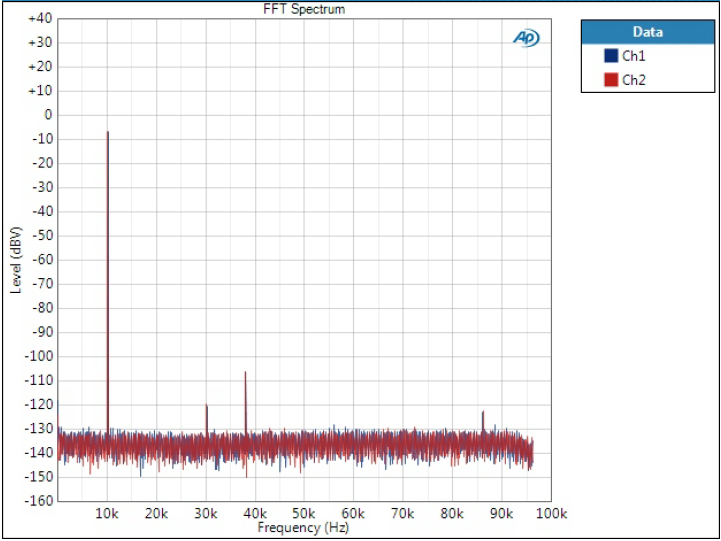
Optimal Spectrum, 10 kHz FFT
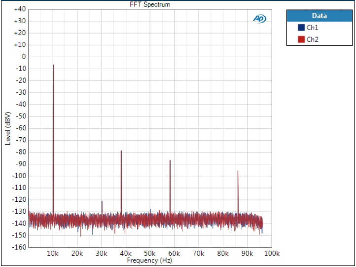
Optimal Transient filters
Optimal Transient, 10 kHz FFT
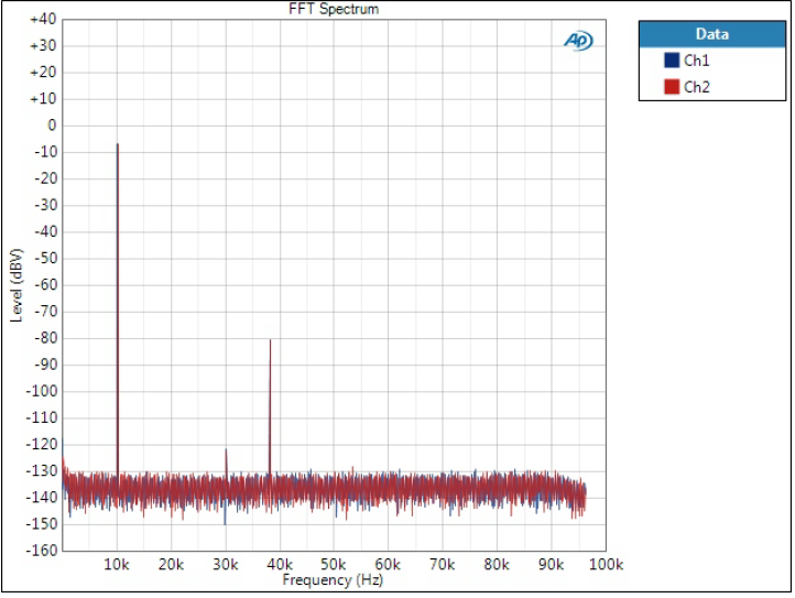
Minimum Phase filter
Minimum Phase, 10 kHz FFT
Sharp rolloff filter
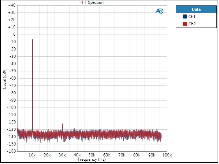
Sharp Rolloff, 10 kHz FFT
Slow rolloff filter
Slow Rolloff, 10 kHz FFT
Sine wave, 10 kHz
Before we had FFTs of 10 kHz sine tone, so how does it look like in time domain? Here we can see how heavily distorted the signal is with filters where the image components are very high.
Only Optimal Spectrum and Optimal Transient are shown as an example. Filters where image components have been attenuated tens of dBs look like pure sine wave to eye.
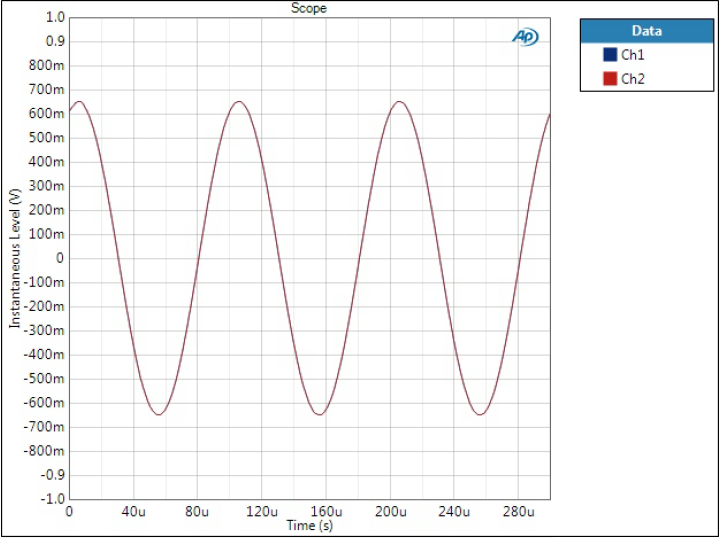
Optimal Spectrum, 10 kHz sine wave
Optimal Transient, 10 kHz sine wave
Does not look like sine wave? When the frequency gets closer to 20 kHz it only gets a lot worse.
One thing to note here is also that sample rate has significant impact on FFTs. With 48 kHz sample rate frequencies get mirrored around 48 kHz so one way to get rid of this is to use higher sample rates.
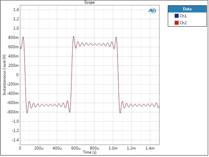
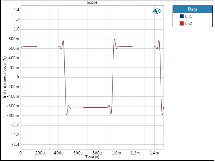
Square wave, 1 kHz
All those spectra and high frequency sine waves make Optimal Transient filters look very bad but this is where they excel. As mentioned in the beginning, time and frequency domains are two sides of the same thing, and optimising one deteriorates the other.
Impulse response is often used to show time domain response of a filter. Unfortunately APx is not the best instrument to show a smooth impulse response without post-processing; therefore, I have used square wave.
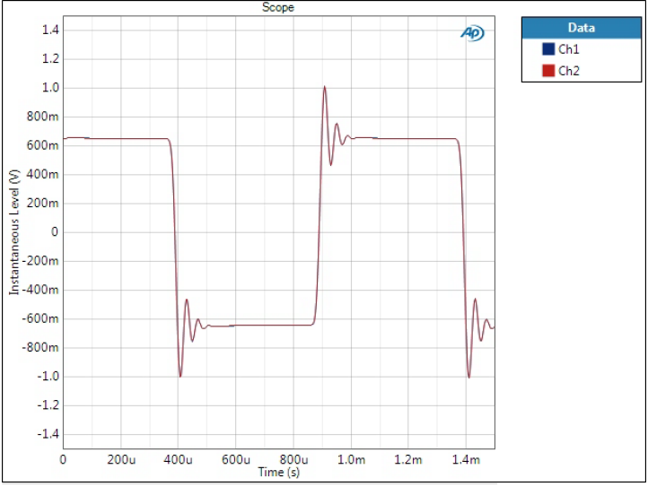
Optimal Spectrum filter
This shows all the possible problems of the before-so-perfect Optimal Spectrum filter. There is quite a lot of ringing and it occurs both before and after the edges. This is usually the tradeoff we need to accept when making otherwise technically great filters.
One major argument against (sorry no reference now but I’m sure any forum will do!) this type of filter is the pre-ringing. After all, it is a phenomenon that happens before something. In the square wave we have an edge coming and the signal starts ringing before the edge. Indeed it appears a bit unnatural.
Optimal Spectrum, 1 kHz square wave
Optimal Transient filters
There is only one Optimal Transient graph here as they look pretty much the same in this scale. Here these filters truly excel – ringing is minimal and edges are sharp. This is of course clear to all familiar with the Fourier series theory; when looking at the spectra one must have higher frequency components present to create a good square wave response.
Optimal Transient, 1 kHz square wave
Minimum Phase filter
Minimum phase shows significant over- and undershoot but ringing time is short. Pre-ringing is also absent here.
Minimum Phase, 1 kHz square wave
Sharp rolloff filter
This looks practically the same as Optimal Spectrum due to similar design goals in frequency domain.
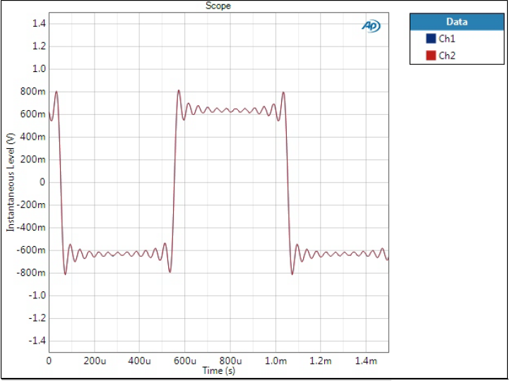
Sharp Rolloff, 1 kHz square wave
Slow rolloff filter
This looks quite different from the rest as well.
Slow Rolloff, 1 kHz square wave
Conclusions
That was quite a lot of graphs – although even more could have been presented. Hopefully this gave an overview what different types of digital filters can do to signal. From a purely technical perspective it can be interesting to examine the filters in time and frequency domains. It gives good representation of basic signal theory without ugly mathematical formulas.
Another thing is of course how it affects the sound. Although measured differences can be significant, the effects on sound are very subtle (in my opinion) and of course subjective. Often I cannot note the difference between the filters and when I can, my preference may vary depending on the type of music. Also, although Optimal Spectrum filters are great engineering tools and technically superb, many listeners may prefer Optimal Transient filters.
I may do more measurements later on but for now the focus will be on other things.
References and additional information
- Internal links
- External links
Version history
This page version history
- 28.1.2019 Initial version
3 comments
Thanks, NIHTILA!
Really thoroughgoing…
I can tell 2 or 3 at most but the graphs are quite distinguishable.
Thanks! Yes the graphs are definitely more distinguishable than sonic differences. At least my ears are not trained enough yet that I could easily point out differences.
Never too late I guess, from John Westlake on the Pink Fish Media forum…
”
What’s interesting about OT and OT XD is that they have exactly the same “Filter” response in both time and the frequency domain, but the results are achieved with differing “Mathematics”.
The difference in “Processing” = Crunching the numbers, modulates the DAC’s silicon die differently (Via Clock and PSU disturbances). You are in fact hearing the effects of a “Second Order” distortion… and the effects are not mild!
OT DD has the same “Filter” response in both time and the frequency domain, but the DAC array is rearranged to Process the Data in a “Balanced Mode” theoretically cancelling or nulling the second order effects in the DAC array… but I still prefer the OT XD filter
Sonically, OT DD has a very different “Bass” (sonically that is, as they measure exactly the same in the Frequency response domain) – I suspect as a result of Balancing the currents within the DAC array. I’d just like to stress that all 3 OT types have the same response in both the time and the frequency domain. I believe that there might be a 0.3dB or so change in amplitude between the OT/OTXD and OT DD (But the responses are the same).”
Comments are closed.