Many DAC chips and devices using those chip have user selectable options for digital filter response to fine-tune tonal characteristics. I will take PCM1794A used on H-DAC as an example and see what effects these filter types have on impulse and frequency responses. This is just scratching the surface of the topic by briefly introducing some technical effects that can be measured. Tonal characteristics are not discussed here; those are highly subjective and a topic of another post (or debate).
An example – PCM1794A DAC IC
TI PCM1794A offers two DAC filter options: slow and sharp. These can be changed with register settings. Below is the filter information found in PCM1794A datasheet. There are frequency responses on the left and their zoomed in versions on the right for each filter type. Frequency axis is relative to sample rate; if we take 48 kHz sample rate as an example, 20 kHz corresponds to 20/48=0.42. What we see from the graphs below is that sharp filter response is flat until 0.45, while slow filter has already more than 1 dB attenuation at 20 kHz. The table also tells that sharp filter has narrower transition band and greater stop-band attenuation but longer delay time.
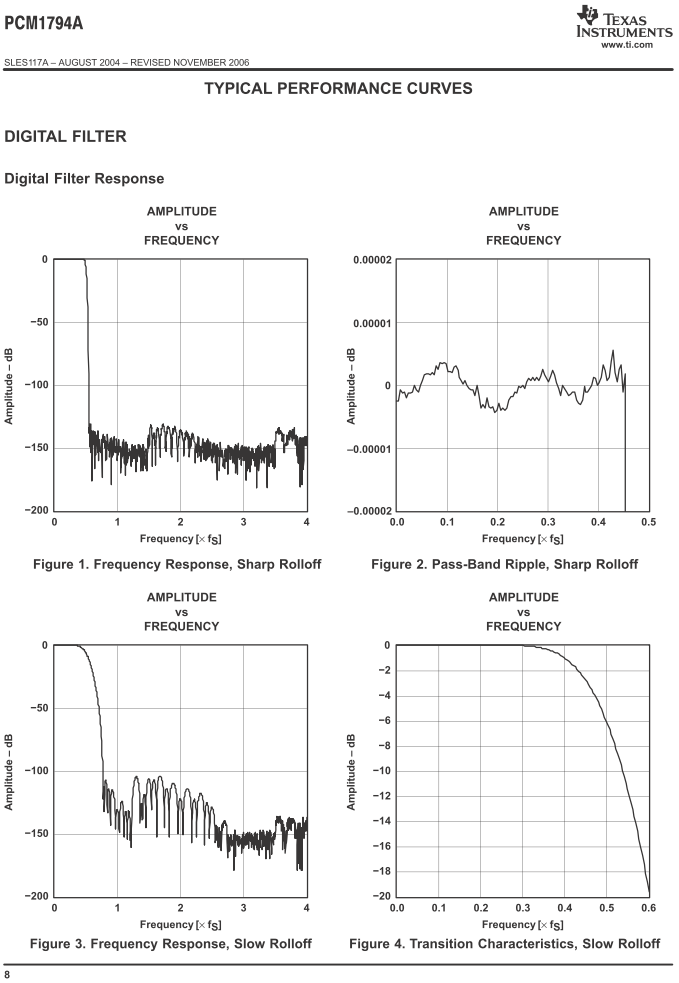
PCM1794A datasheet capture.
Audio band frequency response
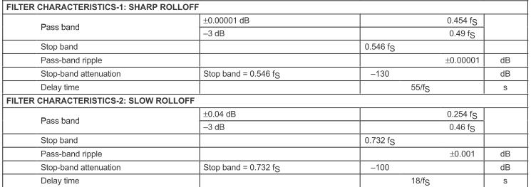
Below are PCM1794A filter responses for 48 kHz and 96 kHz sample rates measured from H-DAC. With 48 kHz and slow filter we see 1.3 dB attenuation at 20 kHz, while sharp filter stays flat until 22 kHz. With 96 kHz sample rate everything is doubled and audio band stays flat with any filter.
H-DAC frequency response with different filters and sample rates.
Impulse response
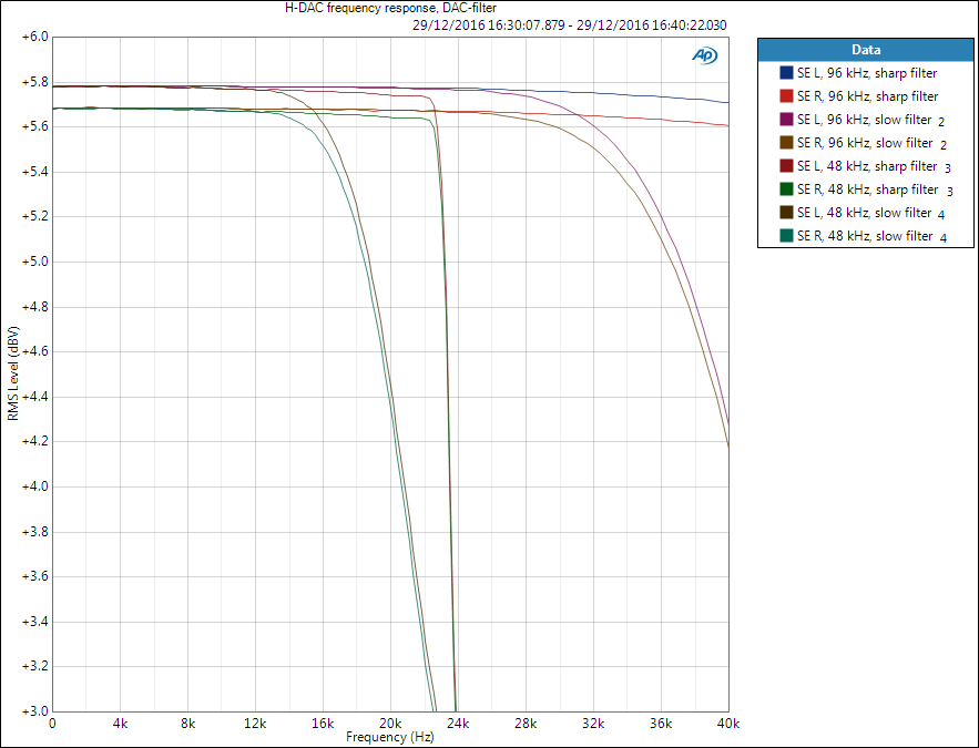
Impulse responses below show the filter effects in time domain. Impulse response is a time domain representation, in a way corresponding frequency response; there is a mathematical relation through Fourier transform. As the name implies, it is the system’s response to an impulse signal and as impulse contains all frequencies, it therefore defines the system response for all frequencies – like frequency response.
In practice impulse is often a tricky signal to generate and measure. Impulse responses below are recorded with APx585 performing a logarithmic sine sweep. The data is interpolated in Scilab for nicer representation.
H-DAC impulse response at 48 kHz sample rate, sharp and slow filters.
When slow and sharp filter impulse responses are compared, denote the following differences:
- Time delay – slow filter is more than twice “faster” than sharp filter
- Amount of pre- and post-ringing – sharp filter has significantly more ringing
- (There are also slight differences in impulse response symmetry but this may be due to data acquisition)
Time delay is proportional to filter length. The more complex the filter is, the longer it is; it requires more taps, meaning the amount of samples the filter processes at one time instant. Steeper filter (higher filter order) is longer, causing longer time delay. Datasheet gives filter delay in samples, as seen in the datasheet captures above: sharp filter is 55 samples long and slow filter 18 samples. At 48 kHz sample rate one sample is 1/48000 seconds. Therefore, sharp filter is 55/48000 = 1.1 ms and slow filter 0.38 ms. Considering other delays in the measurement system, these numbers kind of match the graph above. However, this delay does not really have any direct meaning in a system performance, it is just a technical detail.
Ringing can, however, potentially have effect on audio quality. You can find lots of debates on forums how ringing is bad, especially the pre-ringing. Word “unnatural” is often used as in real world pre-ringing is counter-intuitive; it is caused by something that has not happened yet. Obviously these are opinions and differ a lot. Feel free to link on comments if you find something interesting regarding the topic. This is the reason some people prefer slow filter to sharp one.
Asymmetric impulse response would indicate nonlinear phase response that could in extreme cases change the shape of signal completely.
As everything with digital filters is related to sample rate (in digital system, everything is related to its reference clock), also delays and frequencies change with sample rate. Above we saw corner frequencies doubling when sample rate was doubled, below we see impulse response time delays halving when sample rate is doubled (sample time is halved).
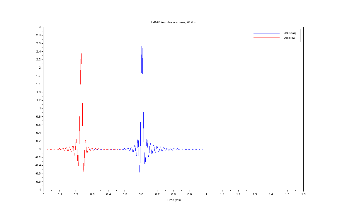
H-DAC impulse responses at 96 kHz sample rate.
Out-of-band spectrum
Let’s get back to frequency domain. Frequency responses shown so far dealt with audio band but what happens beyond that with different filters?
Below is an FFT of H-DAC output with 48 kHz sample rate, sharp filter, and 20 kHz 0 dBFS sine signal. We see the 20 kHz fundamental and harmonics at 40 kHz and 60 kHz which are attenuated roughly 110 dB.

H-DAC out-of-band spectrum, 48 kHz sample rate, 20 kHz tone, sharp filter.
Below is the same situation but with slow filter setting. Now we can see not only the harmonics of 20 kHz but also its image frequency at 28 kHz. If we look at the datasheet filter graphs and realise 28 kHz is around 0.6 in the x-axis, it can be seen that slow filter has only around 20 dB attenuation at that point, while sharp filter possibly has more than 100 dB.
Image frequency is a product of frequency folding, or aliasing, at Nyquist frequency. 48 kHz sampled system has a Nyquist frequency of 24 kHz, meaning 20 kHz signal “folds” over to 24+(24-20)=28 kHz.
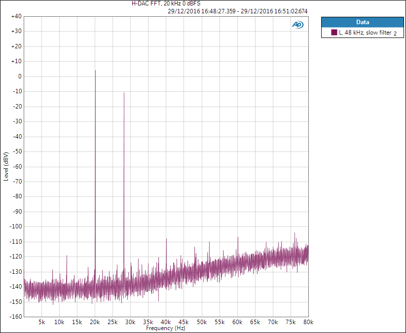
H-DAC out-of-band spectrum, 48 kHz sample rate, 20 kHz tone, slow filter.
If this was given as THD+N figure it would be dreadful. However, these are not shown in normal audio measurements as measurement bandwidth is limited to 20 kHz. Even if we remove it for the measurement, it still does not remove the fact that it is there. Some measurements may feel a bit deceptive as we deliberately mask unwanted effects.
Below is shown the time domain signal. Distortion is very clearly visible as the 28 kHz image is only 6 times smaller than the fundamental. But remember, only at high frequencies – if we had 10 kHz signal, its image would be at 38 kHz where even slow filter has tens of dB attenuation. Therefore, in reality, we do not hear these tones.
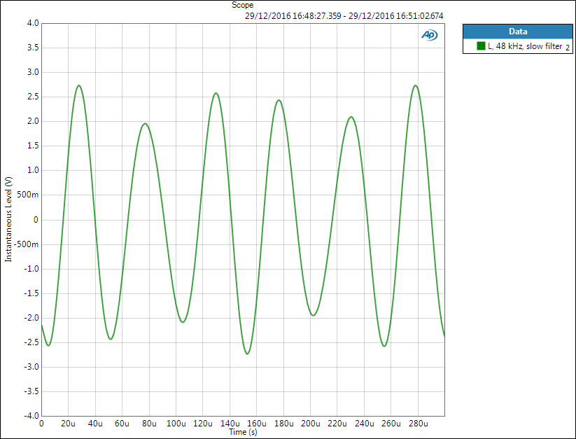
Above signal in time domain.
Next is the slow filter situation with 96 kHz sample rate. These effects are not present with higher sample rates as folding frequency moves higher. In this case the image frequency of 20 kHz would be 76 kHz; it may be the spike seen there at nearly -120 dBV level.
40 kHz and 60 kHz spikes are harmonic distortion.
See the shape difference in noise floor compared to 48 kHz sample rate? Noise shaping is another trick modern DACs use – they move the noise from audio band into higher end of the spectrum. With 48 kHz we see the noise increasing soon after audio band but with 96 kHz it only slowly starts rising within the shown spectrum.
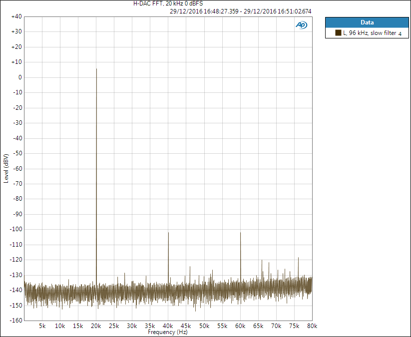
H-DAC out-of-band spectrum, 96 kHz sample rate, 20 kHz tone, slow filter.
Digital filters operating beyond audio band are possible because of over-sampling DACs. By using sharp digital filters and noise-shaping techniques, the DAC is able to remove the nasty high-frequency components or move them to very high frequencies. This significantly eases the requirements for post-DAC analog filter. Back in the times of NOS (non-oversampling) DACs, very steep, bulky, and expensive analog filters were needed to filter out (at least some of) the image frequencies.
Conclusion and final words
To briefly conclude the differences between sharp and slow DAC filter responses:
- Sharp filter; Default option because it is technically superior and one of the reasons oversampling DACs with filters are used. It measures better and requires less from the analog filter at the output, or in some cases it can be left out completely.
- Slow filter; Alternative option. Technically not as good but some claim it sounds more natural. In a way it is a step towards (backwards) NOS DAC.
- NOS DAC without any filter is technically the worst case. However, still some people like the sound of them.
Time and frequency domains are two sides of the same thing. Optimise in one domain and you face a trade-off in the other.
I have shown that the differences between filters can be easily measured. However, their tonal differences are way smaller. In fact, for most (or almost all) they are impossible to hear. I still have to do my own comprehensive tests to see if I can hear the difference. I may come back with another post at a later time. Even if the differences are subtle, it is still good to provide those filter options for the user. As a commercial example I took Audiolab Q-DAC. It has three types of filter settings with following descriptions:
- “Optimal Spectrum: This filter implements sampling theory and is designed for near perfect technical response in the frequency domain.”
- “Optimal Transient: This filter exhibits no ringing and the transient nature of the music is preserved. Although exhibiting ‘lesser’ performance in technical measurements, sound from this type of filter has a purity and ‘naturalness’ that more than compensates for the lack of technical specifications. There are three optimal transient folders which produce identical frequency and time domain response but the internal structure of the filter varies for subtle sonic nuances.”
- “Sharp Rolloff: This filter typifies industrial standard characteristics (-6dB at 1/2 Fs with significant time-domain ringing) and is included here for comparison purposes.”
From what I have shown in this brief post we can make some sophisticated guesses regarding the filters used. “Optimal Spectrum” may be close to the sharp filter shown in these measurements, while “Optimal Transient” is closer to the slow filter setting (probably taken a bit further). The names refer to how their responses look in frequency domain (frequency response – spectrum) and time domain (impulse response – transient).
This is not a simple topic and I am not an expert in digital signal processing but learning at least fundamentals help us be better electronics and audio engineers.
References and further reading:
- PCM1794A datasheet
- “Archimago’s Musings; Measurements: Digital filters and impulse response… (TEAC UD-501)“, blog post on the same topic – check for spectrum image of NOS DAC!
- “The Ayre MP Series“, Ayre paper on digital filters (claims tonal differences between sharp, slow, and minimum phase filters, and also describes negative effects of pre-ringing)
- The Scientist and Engineer’s Guide to Digital Signal Processing
1 comment
[…] Audio Theory […]
Comments are closed.