This post delves into digital filters in AK4490 and AK4493 DACs used in W-DAC boards and provides extensive measurement results of the filters in time and frequency domain. This is not only relevant to these specific DAC chips and filters but general information on DAC digital filters from audio perspective. This is a practical approach – no poles, zeros, or formulas but lots of plots.
I have written about DAC digital filters and their effect in time and frequency domains quite a while ago using PCM1794A as an example. Also M-DAC measurement results discussed how different types of digital filters look in time and frequency domains. However, when I was recording measurements results of W-DAC I got quite good plots again showing effects of digital filters so I thought of revising the topic. For example, I didn’t talk about phase in M-DAC filter post although it is an important part.
Filters under investigation are specific to AK4490 and AK4493 but almost all ICs or devices have at least partly very similar filters. Therefore, this information applies to all audio digital filters to some extent.
Why do we need digital filters?
This is a wide topic but here is just scratching the surface; if you want to know more Google is your friend. Visual representations of oversampling, folding, and image frequencies will help if you’re not familiar with these topics.
Non-oversampling DACs in the past
In early days in CD players we had 44.1 kHz sample rate and non-oversampling (NOS) DACs. If 20 kHz audio band was to be preserved and given Nyquist frequency is 22.05 kHz, we had a very narrow transition band between 20 kHz and 22.05 kHz. As we know from sampling theory and signal reconstruction, if we play 20 kHz tone in such system without any filtering, we will also have 24.1 kHz tone. In order to filter that efficiently, we need a very steep, complicated, and expensive analog filter after the DAC to play back 20 kHz with minimum attenuation and 24 kHz with as much attenuation as possible. There are limitations to this and severe phase shifts will occur.
Oversampling DACs
Basically all DACs (and ADCs) these days oversample; topology like Sigma-Delta is good for high accuracy and linearity, and eases off analog filter requirements significantly. Let’s say our DAC does 8x oversampling. Now the Nyquist frequency becomes 8×44.1/2 = 176.4 kHz but the audio band is still 20 kHz – transition band grows from 2 kHz to 150 kHz and analog filter design becomes significantly easier, simpler, and cheaper.
What happens between 20 kHz and 176.4 kHz? We still have the image frequencies there (e.g. 24.1 kHz when playing 20 kHz) as a consequence of oversampling but digital signal bandwidth is now 176.4 kHz so digital filters can be implemented. What was a task of an analog filter in the early CD player days is now a task of a digital filter. And it is a LOT easier to design a steep tenth order digital filter than analog filter! This digital filter can be designed in numerous ways depending on the design goals. By the original idea we would just make a sharp filter to attenuate as much as possible anything above original audio band of 22.05 kHz.
Non-oversampling DACs now
Anyone browsing diyaudio.com or similar have seen a lot of discussion and debate on non-oversampling (NOS) DACs. Some people seem to prefer how they sound – although being technically.. let’s say mediocre. Audiophiles who use their NOS DACs often oversample their files on PC which is used as a source. That gets rid of the very tight analog filter requirements. For example, using 96 kHz files moves the Nyquist frequency to 48 kHz and that helps a lot! However, essentially this is doing the same thing on PC what an oversampling DAC is doing on silicon. But of course, experimenting can be fun so if you want to try NOS DACs and oversampling on PC, feel free to do so.
There are also ways to try NOS type of sound by using suitable filter such as Super Slow filter shown here. DAC architecture is still not the same so NOS purists would probably say it’s not the real thing.
Filter types
There are numerous filter types and names but for simplicity we can categorise digital filters into sharp and slow. Similarly named filters can be often found in DACs. Alternatively, naming can be related ‘optimal spectrum’ and ‘optimal transient’, respectively, as in M-DAC. If there are more filter options, they often lie somewhere in between.
There are five filters in AK4490, named in datasheet as follows:
- Sharp
- Slow
- Short Delay Sharp (SD Sharp)
- Short Delay Slow (SD Slow)
- Super Slow
AK4493 has these five plus a sixth one:
- Low Dispersion Short Delay
Sharp filters
Sharp filters offer technically great performance and the best measurement results. These filters are steep in frequency domain and effectively filter out high frequency components above Nyquist frequency. One reason to start using oversampling DACs and digital filters was to achieve this behaviour and ease requirements for the analog output filter.
While having clean spectrum, tradeoff is excessive ringing in time domain. This ringing can happen not only after a sharp edge but also before which sounds counter-intuitive – we see the effect of an edge already before the edge. It’s not black magic though but due to long filter length which also delays the signal. We may not see the edge yet but it is already in the filter when we see the pre-ringing.
In AK4490 and AK4493 there are two different sharp filters.
Slow filters
Slow filters are not as steep in frequency domain so more higher frequency components come through. This can lead to heavily distorted signal on the higher end of audio spectrum.
Flipside here is that time domain looks cleaner with sharp edges without excessive ringing.
In AK4490 and AK4493 there are two different slow filters and one super slow filter.
Linear phase filters
Phase defines how different frequencies are delayed in the filter. If delay is not the same for all frequencies, output waveform will not have the same shape as input. If delay is constant across frequency, we call these linear phase filters.
Linear phase filters can be recognised from their impulse response which is symmetric and in practice also longer than non-linear phase filter. This longer impulse response means longer group delay but it usually doesn’t matter in audio.
As W-DAC 4490 has two Sharp filters and two Slow filters, one of each is linear phase and the other not.
AK4490 and AK4493 filter measurements
Sample rate in all measurements is 48 kHz. Things change when using 96 kHz or higher sample rates as original Nyquist frequency moves up and extreme cases are not quite as dramatic as with 48 kHz. Think of it that part of the oversampling has been done already, also gaining some benefits. Thus, especially slow filters benefit from higher sample rate.
Measurement bandwidth is 90 kHz except in some high bandwidth FFTs it is 1 MHz. Cutoff frequency of the 3rd order analog filter in W-DAC is around 100 kHz.
Level of tones is -20 dBFS so there are no harmonics from analog parts.
Note that Ch1 is Left and Ch2 Right but the results are practically identical for both channels.
FFT of noise
FFT of white noise gives indication of the filter slope.
Both sharp filters and both slow filters have identical looking plot so only one is shown.
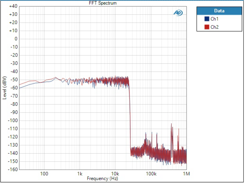
Noise bandwidth of sharp filters
Here we can see how sharp filter transition is between 20 kHz and 30 kHz where we ideally want it to be to have the most efficient filter.
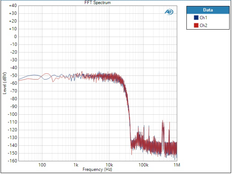
Noise bandwidth of slow filters
Slow shows more relaxed roll-off.
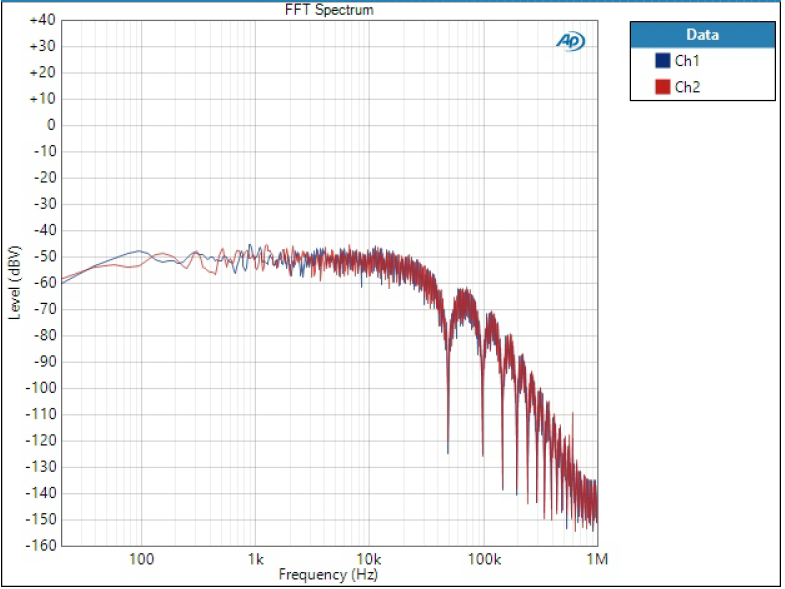
Noise bandwidth of Super Slow filter
Super Slow is something different as we will also see in other measurements.
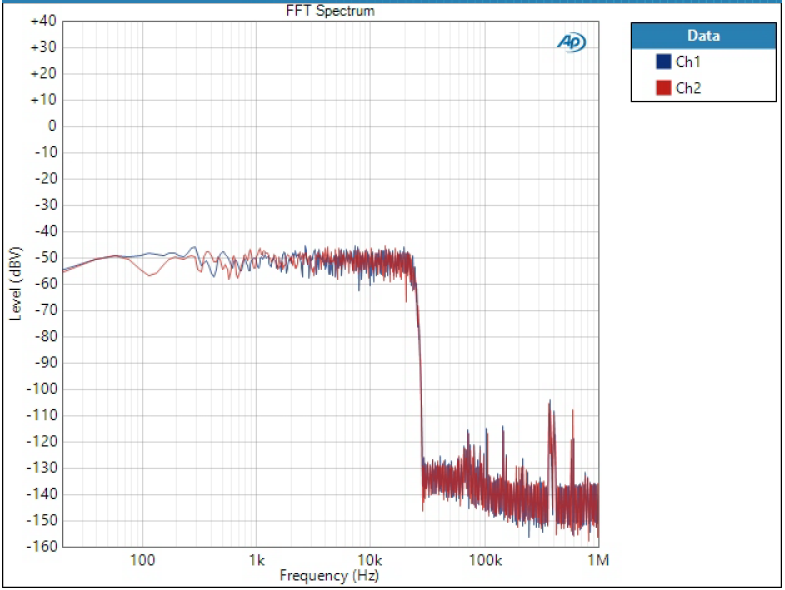
Noise bandwidth of Low Dispersion Short Delay filter
Low Dispersion Short Delay seems to be somewhere between Sharp and Slow.
FFT of 10 kHz tone
10 kHz tone in frequency domain shows how image frequencies are formed beyond Nyquist frequency, following filter envelopes shown in noise FFT above. At 48 kHz sample rate the first image of 10 kHz is at 38 kHz.
Both sharp filters and both slow filters have identical looking plots so only one is shown.
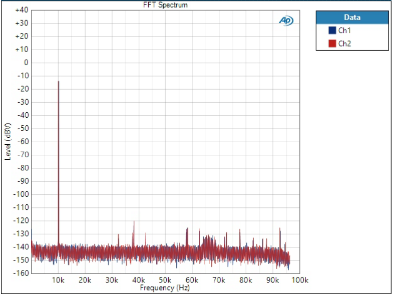
10 kHz FFT of sharp filters
As expected, sharp filters do the best job at getting rid of the image tone.

10 kHz FFT of slow filters
Slow filters show significant spike at 38 kHz.
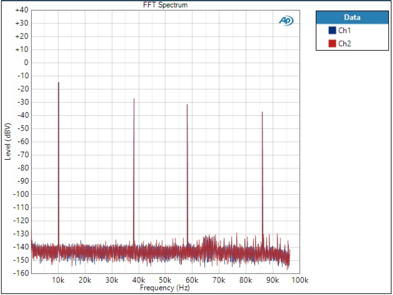
10 kHz FFT of Super Slow filter
Super slow roll-off is as the name implies so all four visible image tones are massive.

10 kHz FFT of Low Dispersion Short Delay filter
Low Dispersion filter does something different but also have significant tones at all image frequencies.
Next, let’s see time domain signals.
Impulse response
Impulse response is one of the most typical characteristics of digital filter although it may tell little to an audiophile. There are few things we can conclude from impulse response:
- Pre-ringing; relative amplitude and length of ringing before the impulse
- Post-ringing; relative amplitude and length of ringing after the impulse
- Phase linearity; symmetrical impulse means linear phase
- Group delay; time delay of the impulse from zero
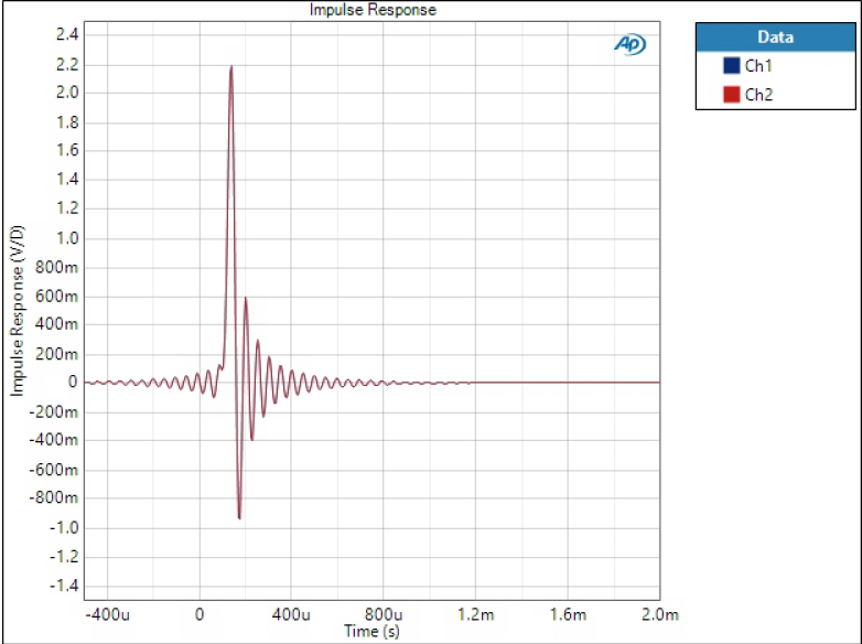
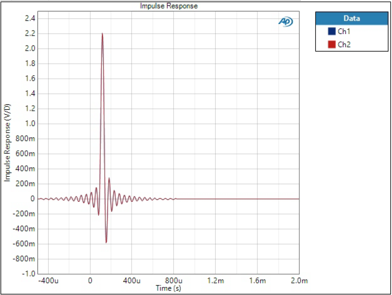
Short Delay Sharp filter impulse response
SD Sharp filter has the highest ringing, especially post-ringing is very high.
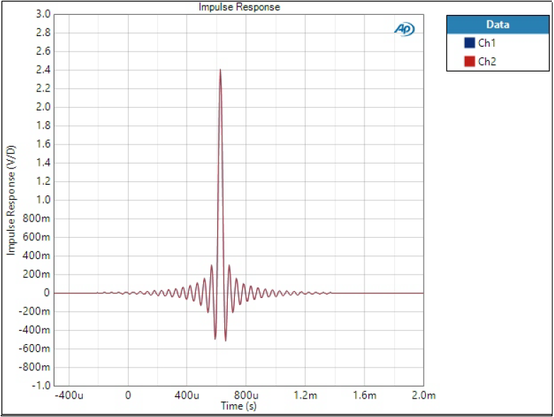
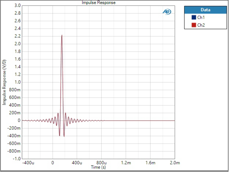
Sharp filter impulse response
Sharp filter has still quite some ringing but less than SD version. Group delay is a lot longer but symmetrical shape tells it’s linear phase filter.
Short Delay Slow filter impulse response
Looks quite similar to SD Sharp but less ringing.
Slow filter impulse response
Phase-linear version of SD Slow; not much difference in group delay though.

Super Slow filter impulse response
Phase-linear, very short group delay.
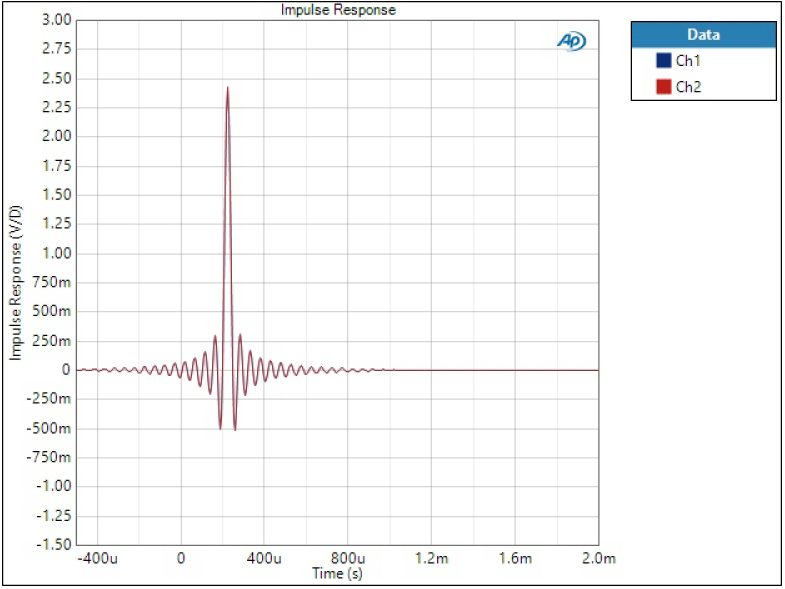
Low Dispersion Short Delay filter impulse response
Looks similar to Slow.
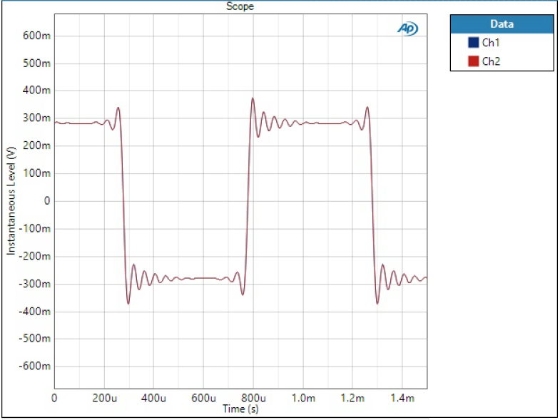
Square wave
Impulse responses may look more or less similar, all having some sort of ringing before and after the impulse. I like to see 1 kHz square wave to better show the characteristics of ringing and sharp edges. Here we can pay attention to a couple of things:
- Pre-ringing; ringing prior to edge
- Post-ringing; ringing after edge
- Over/undershoot; amount edge goes over/under the steady level
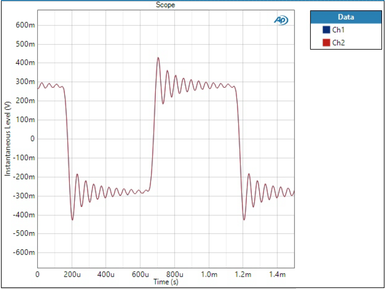
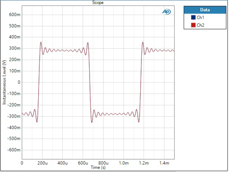
Short Delay Sharp filter 1 kHz square wave
Long and high post-ringing (if there is pre-ringing it may even be masked by post-ringing), and high over/undershoot.
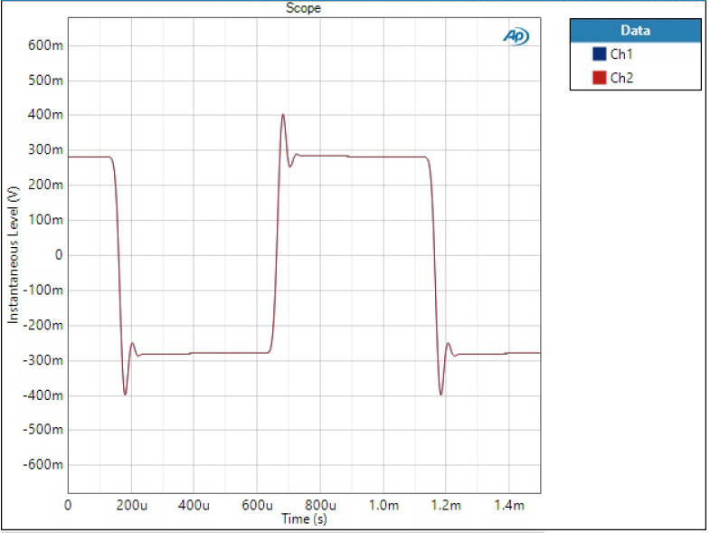
Sharp filter 1 kHz square wave
Significant pre-ringing (ringing starts before edge), overall ringing smaller than in SD sharp, and notable over/undershoot.
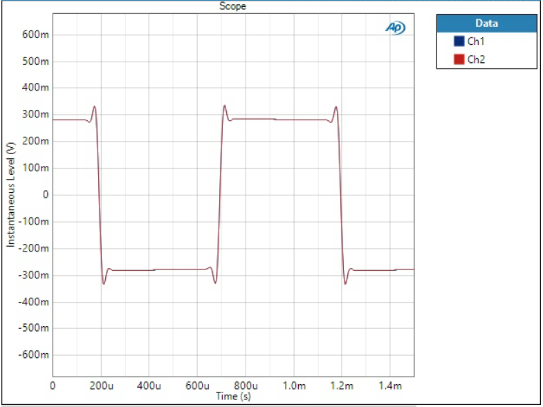
Short Delay Slow filter 1 kHz square wave
These look very different; here ringing is minimal but quite some over/undershoot.
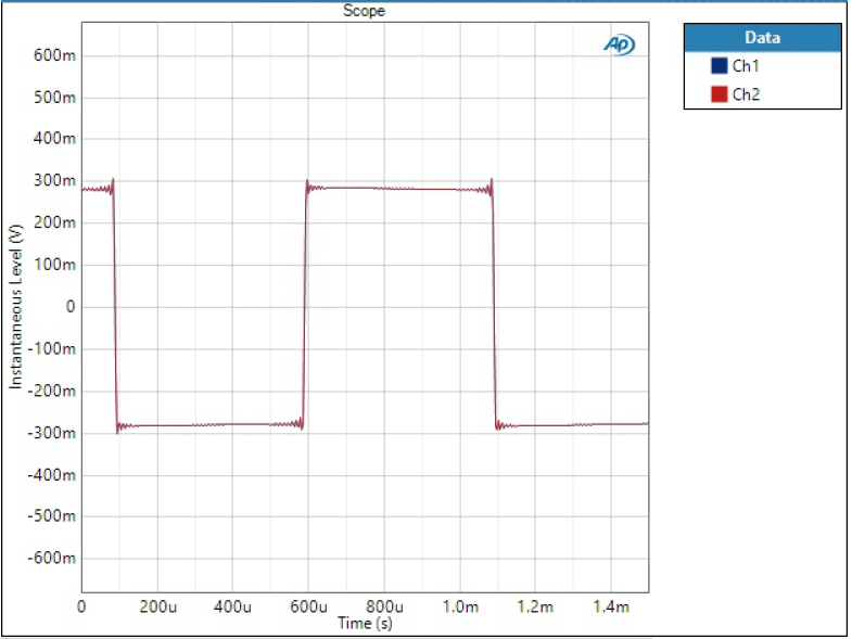
Slow filter 1 kHz square wave
Slow has basically no ringing and only a little bit of over/undershoot.
Super Slow filter 1 kHz square wave
This is quite extraordinary (also) in time domain; only tiny ringing and almost no over/undershoot.
Low Dispersion Short Delay filter 1 kHz square wave
Low Dispersion also looks quite different to anything else; some pre- and post ringing but it decays rather quickly, notable overshoot.
Square wave is the best indication of tradeoff after the 10 kHz FFTs. If we there saw that sharp filters were near ideal in frequency domain and especially Super Slow was absolutely awful, here it is completely opposite. Super Slow shows near ideal time-domain square wave.
Of course this is no surprise considering what square wave is made of (its Fourier series). To reconstruct better square wave, one needs more higher frequency components – and this can be seen in messy spectra of slow filters.
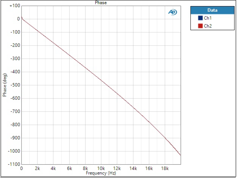
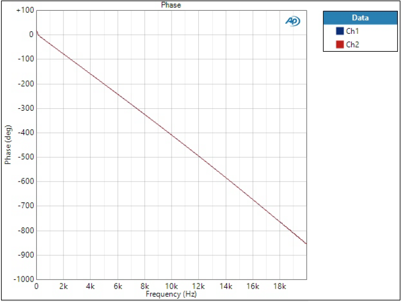
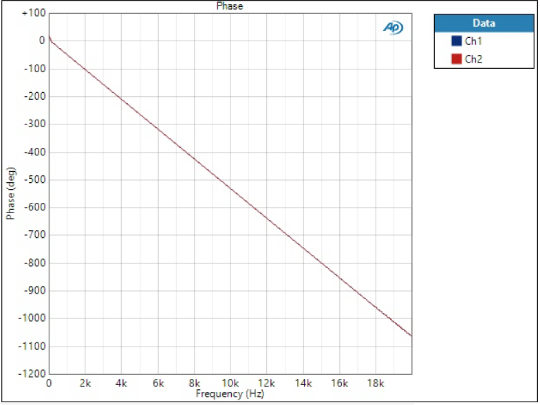
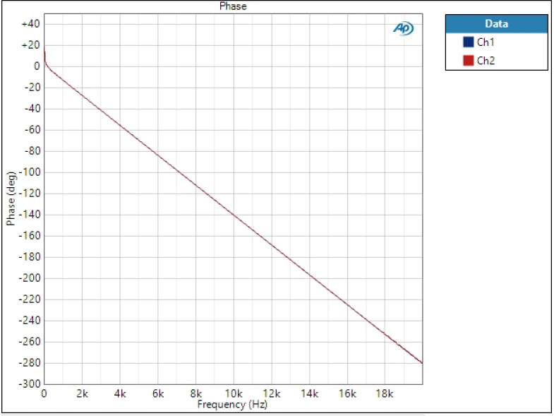
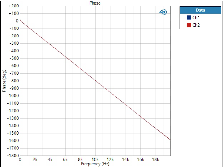
Phase response
Phase is plotted on linear frequency to better see the phase linearity.
Short Delay Sharp filter phase

Sharp filter phase
Short Delay Slow filter phase
Slow filter phase
Super Slow filter phase
Low Dispersion Short Delay filter phase
All of the phases look more or less straight line but after looking at more accurately, we can see that Short Delay filters have slight curvature and phase is not linear – as was concluded in impulse responses.
Having a look at overall phase shift tells something about the filter order. Sharp filter phase shifts 4500 degrees at 20 kHz, while Super Slow at other end is only 300 degrees. The overall shift doesn’t matter per se, it only means longer group delay.
Note: why is this ‘linear phase’ plot straight vertical line then? Phase is essentially time but relatively to the frequency. 180 degrees at 1 kHz is 0.5 ms but at 2 kHz 0.5 ms is 360 degrees. Drawing time (group delay) instead of phase would be constant.
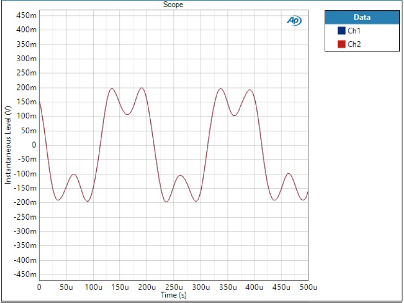
Sum of tones
If phase is non-linear, it means different frequencies have different group delay when going through the filter. This can cause funny effects in practical waveforms. To show this, I have fed a sum of two sine waves through the DAC. The waveform consists of 5 kHz tone at -20 dBFS level and 15 kHz tone half of that level.
Sharp filter is the most optimal in terms of presenting this sort of waveform as it has linear phase response and effectively filters out high frequency components. So this is how the waveform should look like:
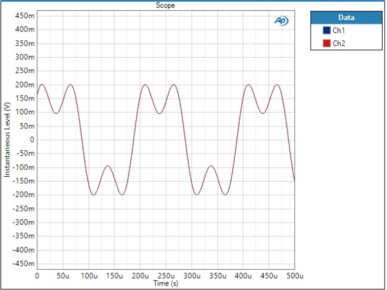
Sharp filter, sum of two tones
The rest will follow:

Short Delay Sharp, sum of two tones
Short Delay Slow, sum of two tones
Slow, sum of two tones

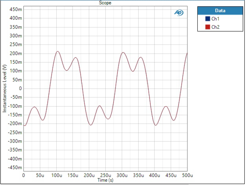
Super Slow, sum of two tones

Low Dispersion Short Delay, sum of two tones
SD Sharp and SD Slow show typical response of non-linear phase filter; output is clean but individual frequency components have different delay causing the sum waveform changing shape.
Slow and Low Dispersion SD filters are almost identical to the ideal Sharp response. These are also phase-linear filters and although they show high spikes on FFT, they are still attenuated so much (remember it’s logarithmic scale) that it’s basically invisible in linear time-domain scale.
Remember how perfect-looking square wave Super Slow filter produced – look at this now. The waveform is awfully distorted due to excessive image frequencies of 5 kHz and 15 kHz tones.
Conclusions
We could say sharp filters are designed for the best technical performance (in frequency domain) and will provide the best measurements results. Sharp filter also provides linear phase but as a consequence has higher delay. SD Sharp achieves similar spectral characteristics but gives away linear phase to achieve shorter latency – tradeoffs, as always.
Slow filters achieve better time domain (transient) characteristics than sharp but as a tradeoff look worse in frequency domain. Again, there is SD version with linear phase although the delay difference is not significant here.
Super slow is a type of optimal transient filter, looking exceptional in time domain but awful in frequency domain.
I must say I don’t know exactly what is the Low Dispersion; it does show characteristics somewhere in between but is still unique.
The best filter?
So what is the best filter then? Such thing doesn’t exist! It depends on your angle of view; do you look at time-domain transient response or spectral purity? How do you value time coherence?
That being said, Sharp filters are often chosen as default and technically superior as these provide the best measurement results and closest follow the signal reconstruction theory. They are the type of filters oversampling made possible and we all should want. But of course it’s never that simple when we’re talking about practical music signal and psychoacoustics. We may not even hear the high frequency images, so should we pay more attention to transient response? For measurement applications you definitely want the Sharp filter with optimal spectrum and linear phase.
If you are more into NOS (non-oversampling) camp, you can try the Super Slow filter. First challenge is of course to hear the differences – it’s not that easy as it looks like on plots.
It’s still worth mentioning that sample rate changes things. Having for example 96 kHz sample rate, Nyquist of slow filters gets higher and they may suddenly look better. Maybe part 3 one day will get back to that.
References and additional information
- M-DAC measurements part 2 – digital filters
- DAC digital filters and their impact in time and frequency domain
- AK4490 datasheet
Version history
This page version history
- 18.10.2019 Initial version
10 comments
Outstanding article!
Thank you for your work. Very informative!
Thanks for this article! It really helped me understand how this all works.
Amazing article. Thank you and I hope you do a part 3 regarding the higher sample rates and how they potentially can put the super slow filter at a more competitive advantage versus the sharp filters.
Thank you for this very interesting and documented article.
I understand better the differences between the filters.
I prefer NOS. Why? Because once the time-domain information is gone, you will never get it back. I consider it essential for spatial definition. Now some people might argue that NOS DACs do less well measuring in the frequency domain, like explained in the article above. But they forget the DAC does not operate in isolation: at some stage the signal will be fed to headphones or speakers. What are headphones and speakers in relation to the DAC? They are low pass filters! So with a NOS DAC we feed a signal with good time domain characteristics but with less good frequency domain characteristics, and our speakers and headphones, through their low pass filtering, will reduces the issues with the frequency domain, especially at higher sample rates such as 96kHz. You might even want to rip your 44/16 CD files and upsample them to 88kHz/24 bits, apply NOS DAC conversion on playback and have even better frequency domain correction than playing NOS at 44/16.
But if you do it the other way around and feed a signal with good frequency domain and bad time domain characteristics, your speakers and headphones will not sort out the time domain issues for you. The baby has already been thrown away with the bathwater.
I do recognise this whole topic becomes a rabbit hole, especially when you take NOS DAC in the mix as well. For now I deliberately kept it to filters. Subjective things are also impossible to write objectively about.
You mention upsampling and then using NOS DAC, in which case you are in fact using some advantage of oversampling. And this is an interesting case and I should maybe write about what Jonathan has mentioned above – using higher sample rates and slow filters. I believe that takes it closer to your example of upsampled files and NOS DAC. This somewhat uses some good bits of both worlds.
Do you have any idea what you are talking about…. Time domain and Frequency domain are co-existing, check Fourier Transform. Basically we have time domain and frequency domain because we measure differently. However, ideally they should be both perfect. So, you said throwing something away… is quite ridiculous…
If you want the math: f=1/T……….. go Google Fourier Transform and its properties.
Hi NIHTILA:
Thank you for this wonderful article, I am also in the EE and physics area… still a student in school. I have a couple questions.
You mentioned:
1. Slow filters:
Slow filters are not as steep in frequency domain so more higher frequency components come through. This can lead to heavily distorted signal on the higher end of audio spectrum.
Can you be a little more specific? Cause if we look at the datasheet or the spec sheet of 4493. Basically slow filter rolls of 6dB from 8khz to 21khz ish. And, I mean beyond 20khz that human beings aren’t able to hear it. So, not sure what do you mean by heavily distorted signal. I mean I did read similar things from Grace design m900, in its user manual. But, I don’t quite get it.
I guess what I meant by distortion there is that if we have a signal that is close to the Nyquist of the used sample rate, images of that will not attenuate very much with slow filters. Then our signal becomes not only the signal itself but the images which can be significant in magnitude if the signal is close to Nyquist. The extreme example of this is the picture of sum of two tones using the Super Slow filter where the signal look very odd.
I do agree this is not as dramatic at all in practice, in fact it can be very very tricky to even notice this in listening tests, even with carefully chosen test signals. And if we use higher sample rates than 44.1k the Nyquist goes way above our hearing range anyway. So take this more as textbook example. I like investigating these from technical perspective but they may not have any meaning in actual listening, or we may even prefer the technically inferior option.
Comments are closed.